If you're looking for simple tricks to make your use of Gaussian98/03 all the easier, I highly recommend heading over to check on the state of Wawrzyniec Niewodniczański's site, larryn.blogspot.com, who's also begun compiling cheat sheets blog-style (which is what I've been trying to do with my site, as it's tough enough to find timely advice and even harder to fumble through online help for a lot of the commercial quantum chemical programs). Wawrzek reminded me that there was at least one semi-useful page from my old site that I forgot to post in the transition to this current site, so here it is (I've not calculated a first hyperpolarizability in four years, but I assume nothing's changed about the formatting).
Lower Triangular Format
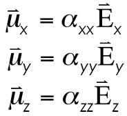
"Lower triangular format" is the means by which Gaussian outputs the components of the 2nd Rank Tensor that is the molecular polarizability. Polarizability is, itself, simply the constant (mostly) by which the induced dipole moment of a molecule is related to the external electric field that is providing the perturbative "nudge" on the electron density. In short, this relationship looks like the following.
![]()
Because dipole moment and electric field are best treated in the general description of molecular polarizability by an orthogonal coordinate system (Cartesian coordinates, for instance) for the sake of simplifying the analysis of dimensional dependence of the electron density from a molecular frame of reference (as opposed to the laboratory frame), the resulting vector treatment of the components of the dipole moment and electric field requires the use of a 2nd Rank Tensor (our way of accounting for a relationship between the interaction of one vector with another). Polarizability, our 2nd Rank Tensor in this general treatment, becomes a 9-component matrix based on all the possible combinations of dipole moment and electric field vectors. The resulting matrix treatment of our simple equation above then becomes the following.

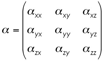
The matrix for alpha is specifically the following.
We begin by simplifying the matrix by utilizing some simple relationships derived elsewhere. In the general treatment of polarizability, it comes to pass that the off-diagonal components of our matrix fall into the following set of equalities.
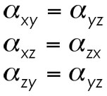
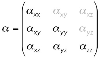
These equalities come from the ability to freely permute the components of the matrix according to the relationship alpha(ab)=alpha(ba). This free perumation stems from symmetry worked out by Kleinman (hence their name, Kleinman symmetry). Therefore, our matrix for alpha above becomes the following.

Because this set of equalities holds, it simply isn't necessary to print the whole mess. Lower triangular format, then, is simply the most basic representation of the polarizability matrix in the order from upper left to lower right read in order. The matrix is treated as the following…
… and the printout of the matrix in Gaussian is
alpha(xx), alpha(xy), alpha(yy), alpha(xz), alpha(yz), alpha(zz)
Editors Note: My thanks to Dr. Andrew J. Alexander, School of Chemistry, University of Edinburgh for catching the reversal of (yy) and (xz) above and Dr. James Kirkpatrick, Experimental Solid-State Physics, Imperial College for catching my text of lower-tetrahedral format but image of upper-tetrahedral format (although, according to the relations we get from Kleinman symmetry, I wasn't wrong, just "less than accurate." Well, I thought it was funny. The image above is correct).
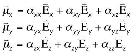
One thing you will likely note in the printout of these values is the rather insignificant value for the off-diagonal elements. These small values stem from the orthogonality of the vectors being considered (what is the dipole moment dependence in the x-direction on an electric field being applied along the y-axis?). The equations for describing the component vector polarizability relations then simplify from…
… to
Within the isotropic limit (molecules basically spherically symmetric, such as Tetrahedral and Octahedral point groups), it can be shown that alpha(xx)=alpha(yy)=alpha(zz). In general, however, the average polarizability of a molecule is calculable as the following (you report the average isotropic alpha even though the values are not rigorously the same. Think of it as simply a good first approximation, as these values will usually be close to one another).
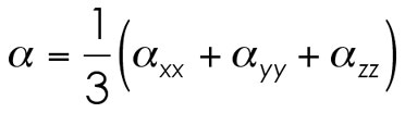
Remember! Average isotropic alpha doesn't mean a vector product. You don't simply apply some trans-dimensional Pythagorean theorem to get the value.This equation looks deceptively like a relation based on the trace (sum of the diagonal elements) of the alpha matrix. Therefore, you may also see this equation written as the following:

Lower Tetrahedral Format
You will probably see this as a natural fall-out of the definition of lower triangular format. I'll hit the high points of the theory regardless to point out some of the subtlties.
First off, beta, or first hyperpolarizability, second-order response, first nonlinear optical response, or one of another of aliases, is a 3rd Rank Tensor. Beta relates how the induced dipole moment vectors (mu(x), mu(y), and mu(z)) are affected by an external electric field along the "a-axis" (a=x, y, or z) AND an external electric field along the "b-axis" (b=x, y, or z). This should make sense as one considers beta to be a value based on two-photon processes (hence the frequency-doubling application of molecules with large first hyperpolarizabilities). A rather awkward way to visualize the matrix description of the induced dipole moment vectors based on the interactions of the two external fields (together) is the following.
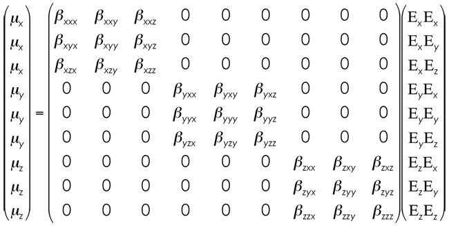
[Yes, I know this is not correct. For those of you that know that, I say that this little simplification does show the high points of the math and gives a simplified view of things in 2 dimensions. For those that don't know (and Nth Rank Tensors are NOT the most common thing in the world), the Nth Rank actually stands for the number of dimensions of the matrix you're playing with. Therefore, a 3rd Rank Tensor is, actually, a cube (in this case, as we're only dealing with the three dimensions). For visualization sake, simply make a cube from the three blocks of betas and throw away the zero's (which are what I'm using to make the math simple). If you're anticipating my picture for second hyperpolarizability (which, yes, means a 4th Rank Tensor), don't hold your breath. Cleaning up this equation, our matrix for beta is simply the following.]

We are again able to freely permute some of the components of beta in the general case of second-harmonic generation (SHG, frequency doubling) by the relation…

… where a, b, and c are any combination of axes ((x,y,z), (x,x,z), etc.). By the cancellation of like-terms and a little catalytic handwaving, our matrix for beta shrinks to the following.

With any luck, lower tetrahedral format now pops out at you as a consquence of the equivalent components being removed. For a pretty interpretation of the "visual" aspect of lower tetrahedral format, check out the following.
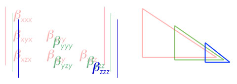
The stacked components of the total matrix create a tetrahedral structure when aligned correctly. Not a pyramid, because each side only has three points to a face. From these 10 unique components of beta, the remainder of the matrix can be solved for.When the actual "vector components" of beta are solved for, equations based on the approximations based on the equailities are common. The value of beta in one of the three axes is calculated from the following general equation.
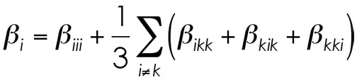
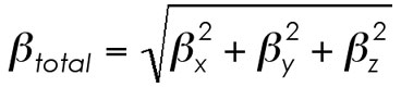
What's happening? This little dance, from the values and symmetry relations defined above, is completed for each dimension (x, y, and z). What you get from this is the first hyperpolarizability of the molecule along that one direction. As you go through the Tensor values, you typically note two major trends. (1) One of the beta(iii) values (xxx, yyy, or zzz) is huge compared to the other two. Orientation along this axis gives the best NLO response and is usually also the axis which the software defines for the dipole moment. (2) The off-diagonal components account for a very small portion of the total beta along one of the axes. Yes, to a worst first approximation, you can simply look at the beta(iii) and get a good idea of what the NLO response of the molecule might be.Finally, when reporting a single value of beta, one of the common formats is to simply treat the three independent values for beta as a quasi-Pythegorean problem and solve for the average beta by doing the following equation (with the square/square-rooting of the values performed to kill any orientational issues that come with the second-order response being positive or negative depending on the orientation of the dipole moment, etc.).
www.gaussian.com
larryn.blogspot.com
www.chem.ed.ac.uk/staff/alexander.html
www.imperial.ac.uk/Research/EXSS/people/staff_ph.asp